5. Example of use

There are plenty of aplications where a RAR dark matter halo can play a role (see the main paper for further details). Here we show a classical application of galactic dynamics, the fitting of a rotation curve.

# =============================== Packages =================================== #
import numpy as np
from scipy.optimize import differential_evolution
import os
from fermihalos import Rar

# Module containing two classes representing an arbitrary disk and an arbitrary bulge
from mass_dist import ExponentialDisk, deVaucouleurs
# ============================================================================ #

# ============================= Observations ================================= #
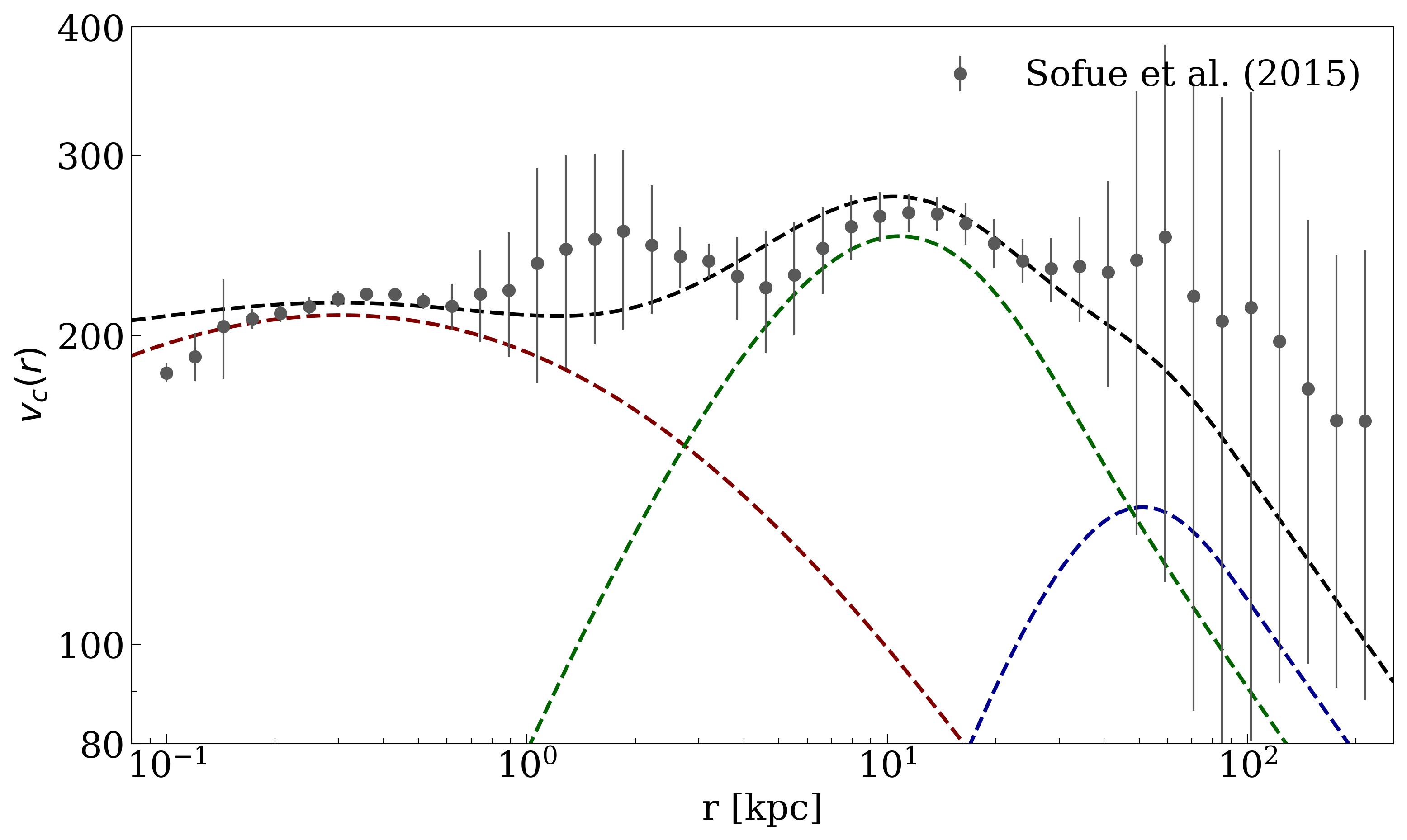
""" The observations were taken from Sofue, PASJ, 67, 4, 2015, 75 """
# ---  radius (kpc), velocity (km/s), standard deviation (km/s)
observations = np.loadtxt('M31_grand_rotation_curve.txt')
radius = observations[:,0]
velocities = observations[:,1]
deviations = observations[:,2]

# The first value of deviations is 0 on the list
deviations[0] = deviations[0] + 4.0          # km/s

# Maximum radii to work with
r_gal_max = 250.0                            # kpc
radius = radius[radius < r_gal_max]
max_idx = len(radius)
velocities = velocities[:max_idx]
deviations = deviations[:max_idx]
# ============================================================================ #

# =========================== Initial parameters ============================= #
# - RAR seed to do the fitting
m_DM = 70.0                                  # keV

# Degeneracy parameter
theta_0 = 36.0

# Cut-off parameter
W_0 = 61.0

# Temperature parameter
beta_0 = 4.3e-3

# Mass of the core and its error
m_core = 1.0e8                               # M_Sun
m_core_err = 0.1*m_core                      # M_Sun

# - de Vaucouleurs bulge parameters - Best fits of Sofue 2015
M_b = 1.7e10                                 # M_sun
a_b = 1.35                                   # kpc
kappa = 7.6695
eta = 22.665

# - Exponential disk parameters - Best fits of Sofue 2015
M_d = 1.8e11                                 # M_sun
a_d = 5.28                                   # kpc

# Initial parameter vector
p_0 = np.array([theta_0, W_0, beta_0, M_b, a_b, M_d, a_d])
# ============================================================================ #

# ========================= Bounds for parameters ============================ #
""" Limits to constrain the parameter space and hence ease the best-fitting procedure """
bounds = ((35.5, 37.5),
        (60.0, 62.0),
        (4.0e-3, 4.7e-3),
        (0.5*M_b, 1.5*M_b),
        (a_b - 0.5, a_b + 0.5),
        (1.6e11, 1.9e11),
        (4.6, 6.0))
# ============================================================================ #

# ====================== Reduced chi squared function ======================== #
def chi_2_red(p):
    # Bulge object
    bulge = deVaucouleurs(np.array([p[3], p[4], kappa, eta]))

    # Disk object
    disk = ExponentialDisk(p[-2:])

    # Dark matter halo object
    halo = Rar(np.array([m_DM, p[0], p[1], p[2]]), circ_vel_func=True, core_func=True)

    # Total circular velocity
    v = np.sqrt(bulge.circular_velocity(radius)**2 + disk.circular_velocity(radius)**2 +
                halo.circular_velocity(radius)**2)

    # Reduced chi squared function
    chi = (np.sum((v - velocities)**2/deviations**2) + (halo.core()[1] - m_core)**2/m_core_err**2)/(len(velocities) - len(p))

    return chi
# ============================================================================ #

# ============================ Fitting function ============================== #
def fit(cores):
    opt = differential_evolution(chi_2_red, bounds, strategy='best1bin', maxiter=150,
                                popsize=75, recombination=0.4, mutation=(0.2, 0.5),
                                tol=1.0e-10, atol=0.0, disp=True, polish=True,
                                x0=p_0, seed=10, workers=cores)

    solution = opt.x
    np.savetxt('best_fit_parameters_for_M31_70kev.txt', solution)
    return solution
# ============================================================================ #

# =========================== Fitting procedure ============================== #
# Number of CPU cores to run differential_evolution in parallel
cores = 10
best_fit_parameters = fit(cores)
print("Fitting procedure completed\n")
print("The best fit parameters are: ", best_fit_parameters)
# ============================================================================ #

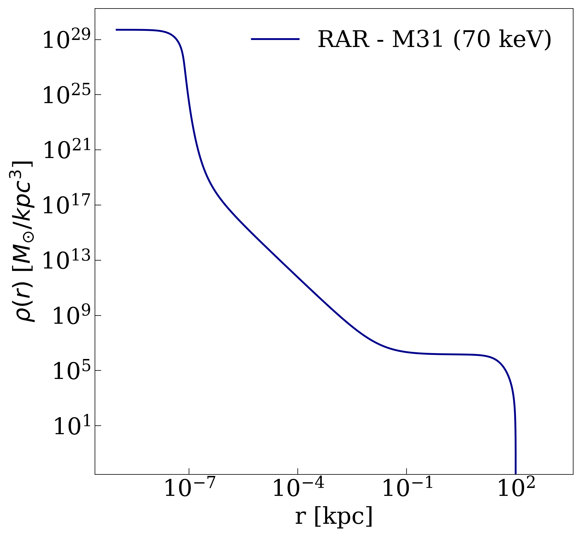
This code will generate a dark matter mass distribution with a radial profile as follows:

and a total circular velocity profile as: